A crypto-perpetual breakout simulation produced 14,399 events across 15 symbols from September 2025 to September 2026. Mean net return was +25.98 bps per event, with a naive event-level t-statistic of +8.20.
But the result depended heavily on how observations were weighted. Returns were concentrated in a small number of market sessions, something the aggregate statistic did not reveal.
Same events, different unit of analysis
I grouped events by calendar day, computed one mean event return per day, then ran a one-sample t-test on those 365 daily means:
event-level:  t = mean(event returns) / (sd / √N)
               = +25.98 / (380.2 / √14,399)  =  +8.20

day-level:    t = mean(daily means)   / (sd / √N)
               = −4.67  / (53.82 / √365)     =  −1.66
These are different estimands. The first weights every event equally; the second weights every trading day equally. The sign reversal does not prove the naive SE was wrong — it shows that the result is sensitive to the weighting choice, which is reason enough to report both. The second is a diagnostic, not a replacement for clustered standard errors or a block bootstrap. For any strategy that fires multiple times a day on correlated moves, it's a useful sanity check.
The day behind the result
October 10, 2025 accounted for most of the positive event-level return. DOTUSDT traded between $0.94 and $4.29 during a market-wide flash crash; ATOMUSDT also experienced extreme price dislocations. Whether the simulated trades were executable at those prices is unclear. The simulation's 434 events that day averaged +835 bps. Remove that one day and the event-level mean changes from +25.98 to −3.69 bps.
The median event lost −16.2 bps. Win rate was 34%. The maximum event return was +8,756 bps. The top 1% of events were enough to flip the mean. Only one day made it positive.
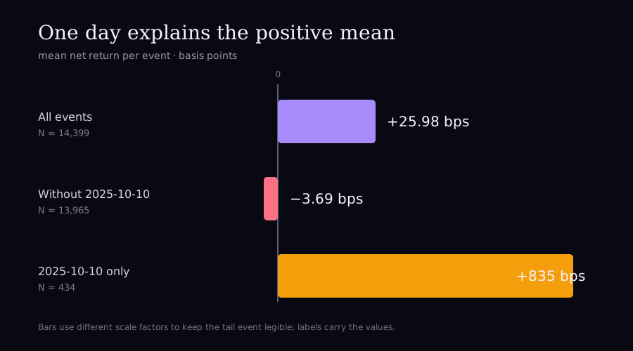
| Statistic | Unit / N | Mean net | SD | t-stat | Note |
|---|---|---|---|---|---|
| Naive t-test | 14,399 events | +25.98 bps | 380.2 bps | +8.20 | Assumes independent events |
| Daily diagnostic | 365 days | −4.67 bps | 53.8 bps | −1.66 | Two-sided p ≈ 0.098 |
| Sensitivity: without Oct 10 | 364 days | −7.37 bps | 14.9 bps | −9.42 | Post-hoc; exposes concentration |
Event-level SD is 380 bps; day-level SD is 54 bps — a 7× collapse. Both t-stats use the same formula (mean / SE), but they're measuring different dispersions. The event-level SE is tiny because N=14,399; the day-level SE is larger because the daily means are themselves variable, and one day (Oct 10, mean +835 bps) inflates both the event-level mean and the day-level SD in opposite directions.
The sensitivity row is not a confirmatory result. Removing an outlier and calling the rerun clean is p-hacking. It is there to show how much of the claim rests on one day.
The diagnostic
Keep the daily series in the result. A t-statistic is one number; the series shows where the result is coming from.
import numpy as np
import pandas as pd
from scipy import stats

def day_block_t(returns_bps: np.ndarray, timestamps: pd.Series) -> dict:
    """Equal-weighted daily diagnostic for event returns.

    Groups events by calendar day, computes the mean return per day,
    and tests whether the distribution of daily means differs from zero.

    This changes the unit of analysis from event to trading day.
    It is NOT a cluster-robust standard error for the event-level mean.
    """
    returns_bps = np.asarray(returns_bps, dtype=float)
    days = pd.to_datetime(pd.Series(timestamps), utc=True).dt.floor("D").to_numpy()
    if len(returns_bps) != len(days):
        raise ValueError("returns_bps and timestamps must have equal length")
    if not np.isfinite(returns_bps).all():
        raise ValueError("returns_bps must be finite")
    frame = pd.DataFrame({"return_bps": returns_bps, "day": days})
    daily = frame.groupby("day")["return_bps"].mean()
    if len(daily) < 2:
        raise ValueError("at least two trading days are required")
    t_stat, p_value = stats.ttest_1samp(daily, popmean=0)

    return {
        "n_events": len(frame),
        "n_days": len(daily),
        "daily_mean_bps": round(daily.mean(), 2),  # input already in bps
        "t_stat": round(float(t_stat), 4),
        "p_value": round(float(p_value), 4),
        "daily": daily,
    }

# Usage
result = day_block_t(event_returns_bps, event_timestamps)
print(f"Event-level t = {event_returns_bps.mean() / (event_returns_bps.std(ddof=1) / len(event_returns_bps)**0.5):.2f}")
print(f"Day-level   t = {result['t_stat']}  (N={result['n_days']} days)")
# Event-level t = +8.20
# Day-level   t = -1.6579  (N=365 days)
Inspecting the concentration
import matplotlib.pyplot as plt

daily = result["daily"]  # already in bps

fig, ax = plt.subplots(figsize=(10, 3))
colors = ["#ef4444" if v > 200 else ("#4ade80" if v > 0 else "#f87171")
          for v in daily]
ax.bar(range(len(daily)), daily.values, color=colors, alpha=0.7, width=1)
ax.axhline(0, color="#6b7280", linewidth=1)
ax.set_xlabel("Trading day")
ax.set_ylabel("Daily mean return (bps)")
ax.set_title(f"Daily mean return — {result['n_days']} days, t = {result['t_stat']:.2f}")

# Flag days > 3σ
mean, std = daily.mean(), daily.std()
outliers = daily[(daily - mean).abs() > 3 * std]
for idx, val in outliers.items():
    ax.annotate(f"{val:.0f} bps", xy=(daily.index.get_loc(idx), val),
                xytext=(0, 8), textcoords="offset points",
                ha="center", fontsize=8, color="#ef4444")
plt.tight_layout()
Leave-one-day-out
Removing October 10 explicitly is post-hoc. The full diagnostic runs the same removal for all 365 days and plots t-stat vs dropped day.
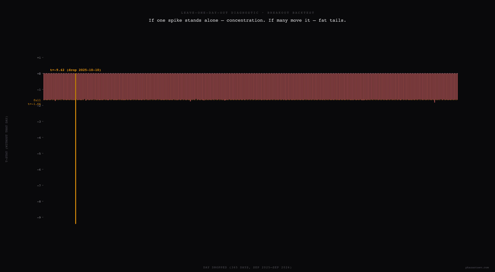
If several days had moved the t-stat materially, the process would be fat-tailed and the right test would be a week-block bootstrap. That's not what happened here: one day, one event cluster, and it's gone when you drop Oct 10.
Limits
There is no single correct return series. If capital is allocated to a portfolio, construct portfolio returns. If the estimand is per-event alpha, preserve that estimand and use an estimator that accounts for dependence: clustered standard errors, a block bootstrap, or HAC/Newey–West where it applies.
Nor is deleting October 10 a valid way to obtain a clean p-value. The primary result keeps every day. The removal is explicitly a post-hoc sensitivity analysis: it tells us how fragile the claim is, not what a pre-specified experiment would have concluded.
The daily t-test still assumes independence across days. It does not automatically account for serial correlation, which is another reason to treat it as a diagnostic rather than the final inference procedure.
The audit found more than dependence: parameter selection on the same data, an optimistic stop-loss simulation, and live feature mismatches. This article isolates the first check because it is cheap to run and easy to miss. In this case, changing the lens from events to trading days stopped a promising-looking backtest from becoming a capital-allocation decision.