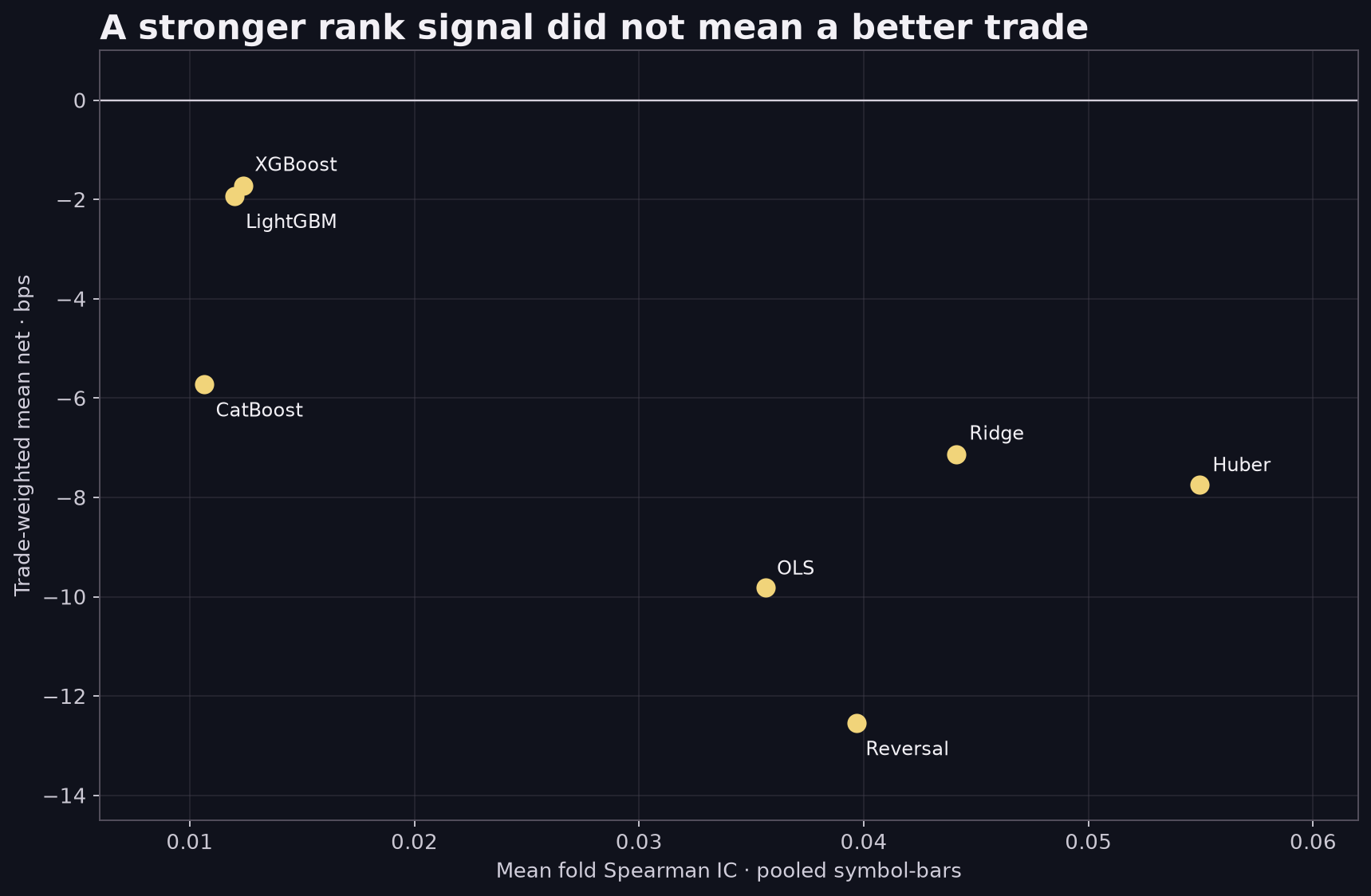
Huber regression had the strongest predictive ranking in this comparison: mean fold Spearman IC +0.055. Its selected trades nevertheless averaged −7.74 basis points after modeled costs.
The least negative result came from one XGBoost configuration, at −1.73 bps per trade, with LightGBM close at −1.93. Both intervals crossed zero. The question that started this project—could LightGBM beat a linear model?—turned into a harder one: what does a better score actually buy us after a trading rule and costs?
An audit of the initial comparison found a fold-boundary leak and gaps treated as consecutive bars. We corrected both and reran the study. Research status: the history was already examined, prices are OHLC proxies, costs are assumed, and the universe was selected retrospectively. This is exploratory research, not a fresh holdout or evidence of a live trading edge.
A signal is not a strategy
The model predicts the next 15-minute return from 1-, 5-, and 20-bar log returns across 16 Bybit perpetual markets. An information coefficient measures rank correlation: does a higher score tend to align with a higher future return? Trading adds a separate question: can the selected moves cover the spread and fees?
Here IC is one Spearman correlation across all available symbol-bar observations in each fold, then averaged equally across folds. It is not a daily cross-sectional IC, and pooled observations can reflect differences between symbols as well as within-symbol ranking. We did not estimate an IC confidence interval in this run.
Why can the rankings differ? IC uses all scored observations to ask about ordering. The trading result uses only the observations beyond a model-specific threshold, assigns a direction and subtracts costs. A model can rank the whole panel well yet select a less rewarding set of extreme scores. The two statistics also weight observations differently, so this experiment does not isolate a single cause of the gap.
The original OLS artifact recorded 4,218 selected historical trades and +5.45 bps mean net under a fixed 12 bps round-trip cost assumption. Its reported bootstrap interval included zero, but an audit found that the implementation dropped repeated sampled days. The interval is unreliable.
| A model metric can establish | It cannot establish |
|---|---|
| Scores rank future returns better than chance | Those returns exceed trading costs |
| A feature relationship repeats across time folds | The relationship survives a threshold and turnover rule |
| OHLC open-to-close proxy P&L | Executable bid/ask fills |
| A positive backtest cell | A best model or a live edge |
One protocol, seven candidates
The learned candidates used the same intended universe of 16 symbols and three return features; the reversal baseline uses the first feature alone. All candidates share six expanding walk-forward folds from 2022 through 2024 and the same next-bar open-to-close outcome proxy. Training begins in 2021 and expands every six months. Symbols enter the panel when their data becomes available; the universe was selected retrospectively and can carry survivorship bias.
The original set contained one-bar reversal, OLS, Ridge, Huber regression and constrained LightGBM. We later added XGBoost and CatBoost in a separate, post-hoc extension using the same splits, inputs, threshold rule and costs. The boosters use fixed, untuned settings, but their tree-building algorithms and effective regularization differ. These are comparisons of individual configurations, not an exhaustive contest between model families.
For the extension, both boosters use 200 trees, depth 4 and learning rate 0.03. XGBoost uses min_child_weight=2000, L1=1 and L2=10; CatBoost uses L2=10. Ridge uses a deliberately strong fixed alpha=1,000,000 on standardized features; its effective regularization changes relative to the growing training sample. A different tuning budget could change this ranking.
Each model's trade threshold was set to the 99th percentile of its training score magnitude. Model scores use different scales, so a shared 12 bps cutoff would give some models more chances to trade for reasons unrelated to prediction quality.
Finally, every selected trade paid the same assumed round-trip cost schedule: 13 bps for BTC and ETH, 15 bps for SOL, XRP, DOGE and BNB, and 19 bps for the rest. That is 5.5 bps taker fee per side plus 1, 2 or 4 bps assumed slippage per side. These are modeled inputs, not observed historical fills or a guarantee of actual fees.
| Protocol | Implementation in the corrected run |
|---|---|
| Features / label | Log returns over 1, 5 and 20 consecutive 15-minute bars; next-bar close-to-close return in bps |
| Decision / outcome | Long above the 99th percentile of absolute training scores; short below its negative; next-bar open-to-close proxy |
| Model settings | OLS; Ridge alpha 1,000,000; Huber epsilon 1.35, alpha 0.0001; LightGBM 200 trees, depth 4, 15 leaves, 2,000 minimum child samples |
| Aggregation | Equal-fold mean Spearman IC; trade-weighted mean net bps, with equal-fold net shown separately |
The percentile comes from in-sample scores. It does not force every model to select 1% of future bars. The reversal baseline scores negative one-bar log return in return units; learned models score predicted bps. Each uses its own training distribution to define its cutoff, so trade counts and future exposure can still differ.
The experiment in five equations
Let C[t] and O[t] be the close and open of bar t. A row is kept only if the required 20 preceding intervals and the following interval are continuous. All model and scaler fitting happens within the expanding training window.
features:    x[t, k] = log(C[t] / C[t-k]),  k ∈ {1, 5, 20}
train label: y[t]    = 10,000 × (C[t+1] / C[t] − 1)
threshold:   q       = 99th percentile of |score| on training rows
signal:      s[t]    = +1 if score > q; −1 if score < −q; else 0
proxy net:   p[t]    = s[t] × 10,000 × (C[t+1] / O[t+1] − 1) − cost
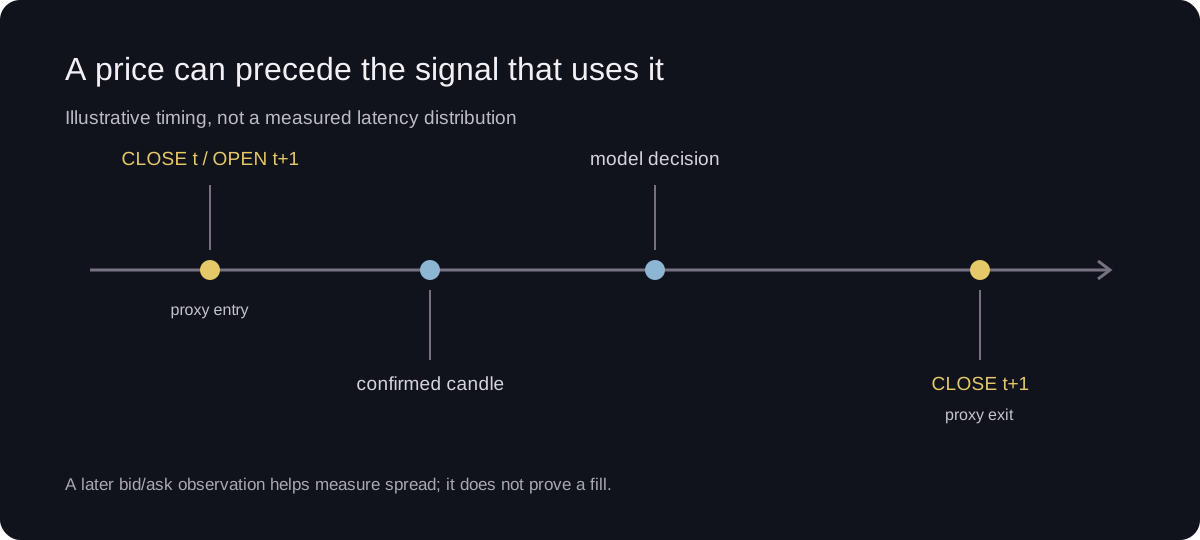
The final equation applies only to selected trades, where s[t] is nonzero; inactive bars do not incur a trade cost. The model learns close-to-close return, while the economic proxy measures open-to-close in the following bar. The next open can occur before a real system reacts to a confirmed close, so the OHLC price does not establish that a trade could have filled there. A basis point is one hundredth of one percent of position notional.
The corrected result
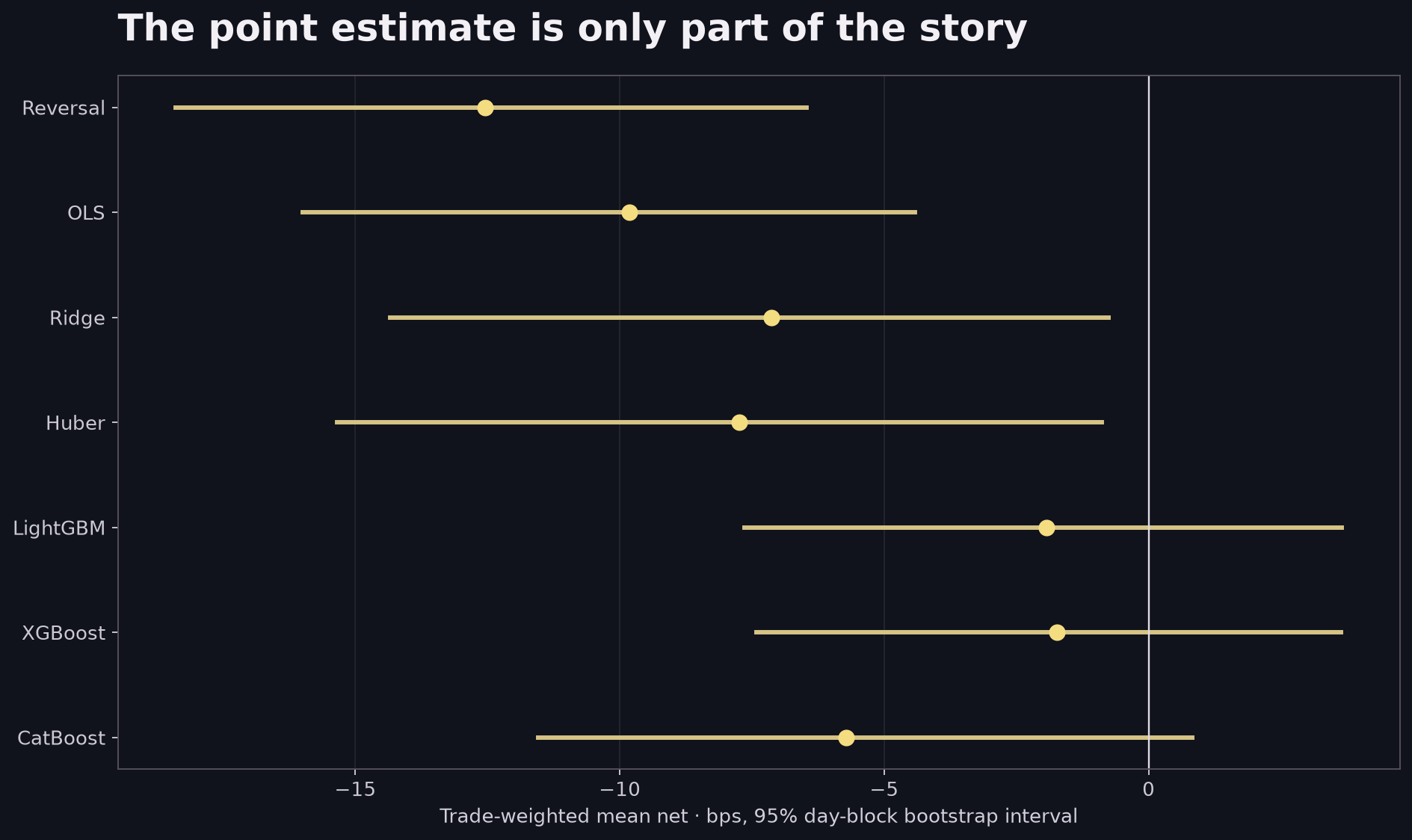
Huber had the highest mean fold IC. Of these seven fixed configurations, XGBoost had the least negative trade-weighted mean, narrowly ahead of LightGBM. Both estimates have wide intervals that cross zero. These are descriptive rankings; the data and candidate selection were already exposed to previous research.
| Model | Mean fold IC | Trade-weighted net | 95% block interval | Trades |
|---|---|---|---|---|
| XGBoost* | +0.012 | −1.73 bps | [−7.41, +3.63] | 10,885 |
| LightGBM | +0.012 | −1.93 bps | [−7.64, +3.65] | 11,006 |
| CatBoost* | +0.011 | −5.73 bps | [−11.54, +0.83] | 11,341 |
| Ridge | +0.044 | −7.14 bps | [−14.34, −0.76] | 12,685 |
| Huber | +0.055 | −7.74 bps | [−15.34, −0.88] | 12,487 |
| OLS | +0.036 | −9.82 bps | [−16.00, −4.42] | 12,461 |
| One-bar reversal | +0.040 | −12.55 bps | [−18.39, −6.48] | 11,497 |
*XGBoost and CatBoost were added after the initial comparison. Parameters differ between implementations; none were tuned in this extension. “Out-of-sample” here means out of each fold's fitting window, not a clean final holdout. Positive IC values are descriptive averages, without a statistical significance claim.
Trade-weighted net sums selected trade outcomes across folds and divides by their count. An equal average of the six fold means answers a different question: for LightGBM it is −3.09 bps. Neither measure is a portfolio return: the backtest does not normalize simultaneous positions, capital, exposure or turnover.
The intervals use 2,000 resamples of contiguous 10-calendar-day blocks, preserving all selected trades on a sampled day together. The resampling holds fitted models and their selected trades fixed; it does not refit the models. LightGBM's interval spans zero; it does not establish profitability or rule it out. These intervals depend on the block choice, do not capture model-selection uncertainty, and are not adjusted for multiple comparisons.
Look inside the average
The six columns show mean net bps per selected trade for each half-year, from 2022 H1 to 2024 H2. Results vary substantially across periods.
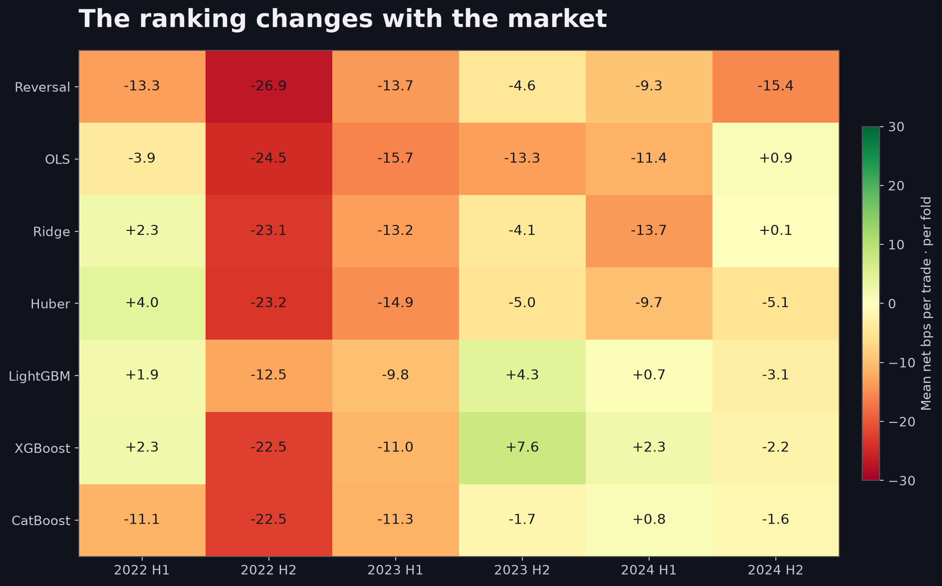
LightGBM's three positive fold means are small beside its two largest negative folds. Huber's stronger average ranking metric does not translate to a better trade-level average under this rule. In paired day-block resampling, the estimated LightGBM-minus-OLS difference has a 95% interval of [+3.71, +12.90] bps per trade. That is an exploratory comparison of different selected trade sets, not an adjusted claim of a general model advantage.
What happens when positions share capital?
The table weights each trade equally. A model that selects many simultaneous markets could therefore look different when those positions have to share capital. We ran a separate, post-hoc portfolio proxy: on every active bar, divide 1× gross notional equally among the selected symbols, enter at the next open, exit at that bar's close, and charge the same assumed round-trip costs. When there is no valid selected signal, the proxy holds cash.
With the original in-sample threshold, the mean daily additive proxy is −53.68 bps for LightGBM and −54.62 bps for XGBoost. LightGBM has the less negative number under this aggregation, reversing their per-trade ordering. The paired 10-day block-bootstrap interval for XGBoost minus LightGBM is [−14.95, +11.59] bps per day: it includes zero.
Does the threshold matter?
The original 99th percentile is calculated from predictions on the same observations used to fit each model. As a sensitivity test, we fit a second model on the first 80% of each outer training window, purge labels crossing the boundary, and calculate the percentile from predictions on the remaining 20%. We then refit on the full outer training window and apply that held-out threshold to the evaluation fold. This is one post-hoc chronological split, not a tuned or independently validated rule; refitting can change the score scale.
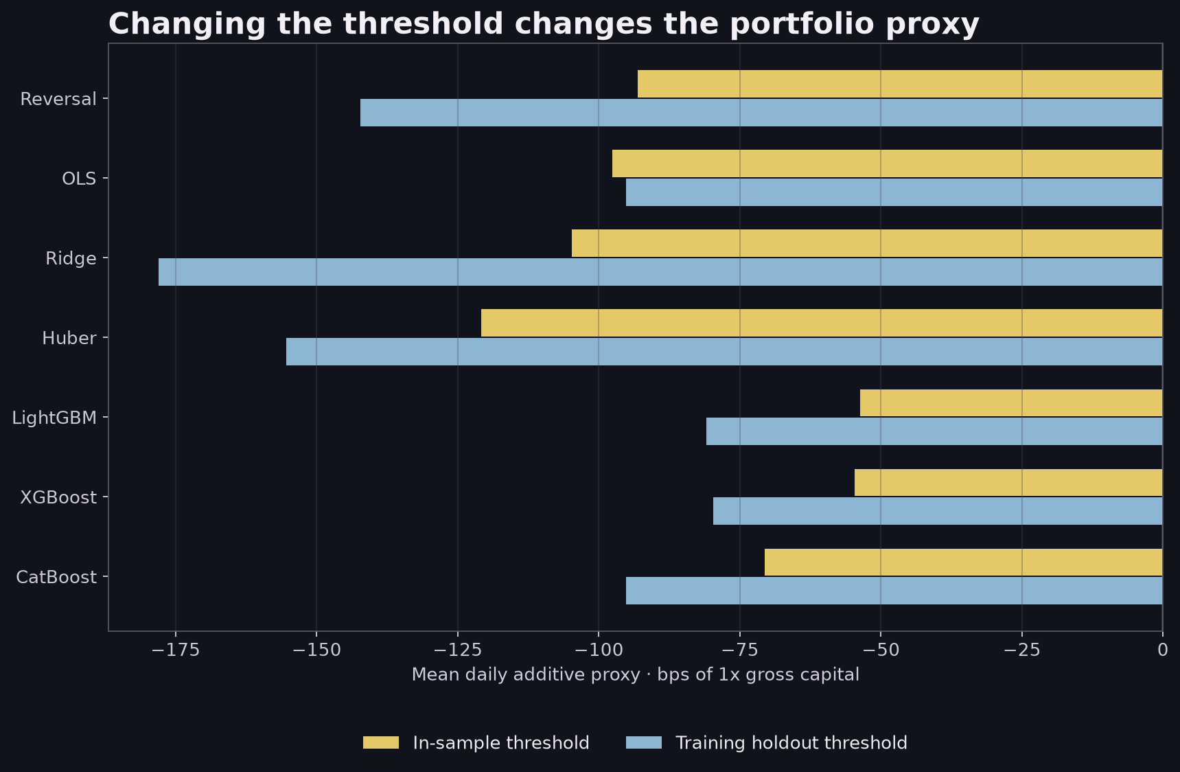
With the training-holdout threshold, LightGBM's mean daily additive proxy changes to −80.98 bps and XGBoost's to −79.67 bps. Their ordering switches again. The paired interval for XGBoost minus LightGBM is [−12.15, +13.46] bps per day, again including zero. Both intervals use 2,000 resamples with the same 10-day blocks across models. The models are not refitted in the bootstrap, the historical period was already examined, and neither interval is adjusted for multiple comparisons.
These are sums of bar-level bps assigned to the next-bar entry day and divided by calendar days, including days in cash, with notional reset to 1× whenever a signal is active. They are not compounded account returns. The proxy does not model funding, impact, order-book depth, margin, liquidation, or changing equity; it treats missing or invalid symbol-bars as unavailable signals. Equal gross notional is also not equal risk. The calculation answers a narrower question than an executable portfolio backtest.
The cost cliff
For the original five candidates, we kept the selected trades fixed and scaled the entire assumed round-trip cost. LightGBM's mean gross proxy was +16.15 bps; its mean assumed cost was 18.08 bps. The result is −1.93 bps at baseline cost, +7.11 at half that cost, and −20.01 at double cost.
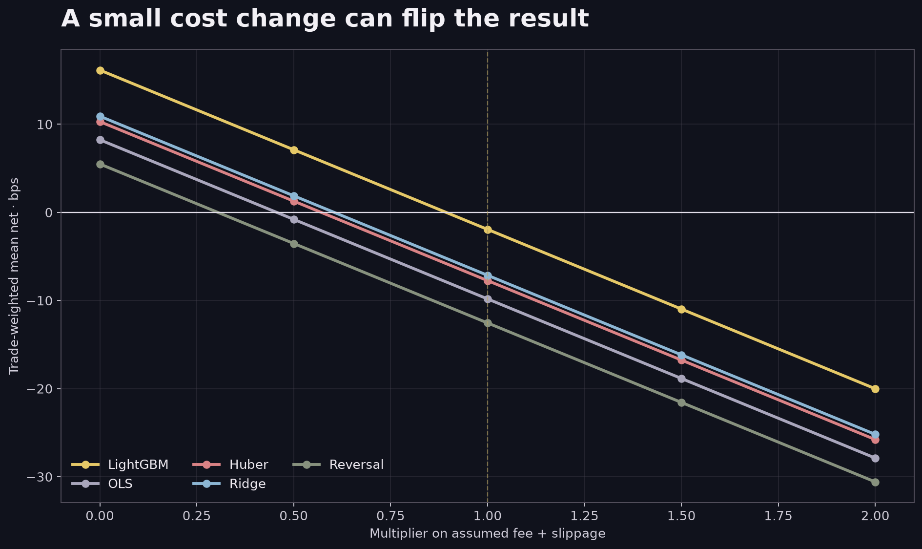
The mechanical break-even multiplier is about 0.89 for this LightGBM trade set: 16.15 / 18.08. It is an arithmetic threshold, not an obtainable fee quote. It ignores uncertainty, execution delay, market impact and any change in behavior caused by a different execution method.
To put the units in context: on a hypothetical $10,000 position, one basis point is $1. The LightGBM averages correspond to roughly $16.15 gross proxy, $18.08 assumed costs and −$1.93 net per selected trade. Those are scaled averages, not cash flows from a funded account; actual position sizes, simultaneous trades and fills are not modeled in that calculation.
Changing the bootstrap block from 10 days to 5 or 20 also left LightGBM's interval crossing zero: approximately [−7.86, +3.83] and [−7.88, +3.80], respectively. This is a narrow sensitivity check, not proof that the interval is robust to every dependence structure.
Why the old OLS result looked better
The previous OLS study and this tournament answer different questions. It used a fixed ±12 bps decision threshold and a fixed 12 bps cost. The tournament calibrates each decision rule inside each training fold and applies tiered 13/15/19 bps costs. Neither convention is the market itself; the point is that a small apparent edge changes sign when the economic contract changes.
Because both the threshold and costs changed, this comparison cannot isolate which change caused the difference. It does show why model comparisons must carry their decision and execution assumptions beside the score: a positive result under one contract does not automatically transfer to another.
What failed the first audit
Fold boundary leakage. The first script assigned training rows by their timestamp but computed each label from the next row. A last training observation could therefore use a price from the evaluation period. The corrected split requires each training label to finish by the evaluation boundary; a regression test changes future prices and verifies that training data remains unchanged.
# Bar timestamps denote bar opens; label_end is the next bar's close.
train = panel[(panel.ts >= train_start) & (panel.label_end <= eval_start)]
eval_ = panel[(panel.ts >= eval_start) & (panel.label_end <= eval_end)]
The important comparison is the end of the label against the evaluation boundary, not merely the timestamp on the feature row. This rule matches this specific next-bar target; a longer holding period or overlapping labels would need their own purge.
Missing bars. The first script used row shifts without verifying a continuous 15-minute grid. The corrected run requires 20 consecutive past intervals and one consecutive future interval, and rejects invalid prices and timestamps. Across the loaded history it detected 1,631 gaps and excluded 34,587 rows, including initial warm-up and incomplete outcomes. Exclusions and file hashes are recorded per symbol in the downloadable results.
Selection and uncertainty. This history was examined in previous research. Candidate and universe selection cannot be treated as a fresh preregistered test. The equal-gross portfolio proxy, threshold sensitivity and paired portfolio intervals were added after inspecting the original results; no multiple-testing correction was computed. They are diagnostics, not confirmation.
Reproducibility. Download the code and result bundle and read the reproduction instructions. We reran all seven models from the extracted bundle against the original files and reproduced the reported aggregates. The bundle also includes a downloader for Bybit's public API and a manifest that checks the original timestamp, open and close values, including missing bars. We independently downloaded and verified all 140,255 BTC rows in the research slice, and checked 1 January 2024 for all 16 symbols (96 bars each). The other 15 symbols have not yet been downloaded in full. The downloader stops if available historical values differ from the manifest.
What happens next
The next step is an executable-price simulation with point-in-time universe rules, realistic order sizing and a portfolio risk model. The simple equal-gross proxy is only a first sensitivity check.
If you are building a similar comparison, keep three questions separate:
- Can the score rank returns? Compare models on the same untouched time windows, and state whether IC is pooled or cross-sectional.
- Does the decision rule survive costs? Freeze the threshold, timing, sizing and fee assumptions; report gross and net results together.
- Would the portfolio have been executable? Check simultaneous exposure, missing data, available liquidity and actual decision-to-order timing. An OHLC open is not a fill.
This experiment answers the first two only under its stated historical assumptions. It does not establish the third.
Separately, we froze seven fitted candidates and specified a new prospective shadow period from 1 November 2026 to 1 February 2027 UTC. The primary comparison is LightGBM versus OLS; the other candidates are secondary. As of 30 October 2026, the period had not started. Collection uses the same exchange and a local process, so this is a new time period, not an external independent audit. A separate observer will record post-decision bid/ask references with a 500 ms minimum delay and mark missed quote windows. Those quotes, like the OHLC proxy, cannot prove an actual fill.
Before the prospective test, we checked the public Bybit top of book during a short collection window on 29 October 2026, 14:30–18:00 UTC. The collector recorded 224 confirmed symbol-bars across 16 markets; 222 had a retained bid/ask snapshot. Median quoted spread across those snapshots was 1.06 bps. Median receipt of a confirmed candle was 724 ms after its scheduled boundary on our host clock. These figures are a small pre-forward diagnostic, not a representative execution estimate: the quote can precede a decision, local clock error affects the delay, and no order was sent. The diagnostic summary reports counts by symbol.
Separately, between 18:57 and 18:59 UTC on 29 October, we submitted five 0.001 BTCUSDT market-order round trips to Bybit's demo environment. In the first, simulated fills were 80,851.8 USDT on entry and 80,845.9 on exit; fees totalled 0.08893374 USDT. All five closed with a loss of between 0.08730960 and 0.10012708 USDT including fees and the price move while holding each position. The anonymized records include pre-entry quotes and execution timestamps. This short, one-symbol demo sample contains no model signals: it is not a representative cost estimate, evidence of live fills, or validation of the historical backtest.
A separate demo-only pilot is configured to attempt at most one 0.001 BTCUSDT round trip per primary model on eligible forward signals, sequentially on a shared account. It can stop for manual review, and connectivity failures can leave a demo position open. Signals can be missed, and the two trades are neither paired nor a statistically useful comparison. Demo fills are simulated; they cannot establish live execution. The pilot does not change the primary shadow protocol.
References
For the model families, see the original papers on LightGBM, XGBoost and CatBoost. For time-aware validation, see the scikit-learn time-series cross-validation example; its gap illustrates the general need to respect when outcomes become available, though our label-specific purge is implemented separately.